Dynamics of size spectra
Size spectrum dynamics
In previous tutorials we have concentrated on the steady state of the mizer model, where for each size class and each species, the rate at which individuals grow into the size class balances the rate at which individuals grow out of the size class or die, thus keeping the size spectrum constant. In this tutorial we explore the dynamic that takes place when this balance is changed.
Size-spectrum dynamics is described by the beautiful partial differential equation
\frac{\partial N(w)}{\partial t} + \frac{\partial g(w) N(w)}{\partial w} = -\mu(w) N(w)
together with the boundary condition
N(w_{min}) = \frac{R_{dd}}{g(w_{min})},
where N(w) is the number density at size w, g(w) is the growth rate and \mu(w) is the death rate of individuals of size w, w_{min} is the egg size and R_{dd} is the birth rate. Luckily it is easy to describe in words what these equations are saying.
Size spectrum dynamics is very intuitive: The rate at which the number of individuals in a size class changes is the difference between the rate at which individuals are entering the size class and the rate at which they are leaving the size class. Individuals can enter a size class by growing in or, in the case of the smallest size class, by being born into it. They can leave by growing out or by dying.
What makes these seemingly obvious dynamics interesting is how the growth rate and the death rate are determined in terms of the abundance of prey and predators and the feeding preferences and physiological parameters of the individuals. We have discussed a bit of that in previous tutorials and will discuss it much more in upcoming tutorials. We will discuss the birth rate R_{dd} below in the section on how reproduction is modelled. But first we want to look at the results of simulating the size spectrum dynamics.
You will be doing your own work for this tutorial in the accompanying worksheet file “worksheet5-dynamics-of-spectra.Rmd”. You will find this file in the worksheet repository for this week that you already used in previous tutorials.
As always, we start by loading the mizerExperimental package as well as the tidyverse.
Projections
In the previous tutorial, in the section on trophic cascades, we already simulated the size-spectrum dynamics to find the new steady state. But we only looked at the final outcome once the dynamics had settled down to the new steady state. We reproduce the code here:
# Create trait-based model
mp <- newTraitParams() |>
    # run to steady state with constant reproduction rate
    steady() |>
    # turn of reproduction and instead keep egg abundance constant
    setRateFunction("RDI", "constantEggRDI") |>
    setRateFunction("RDD", "noRDD")
Convergence was achieved in 6 years.# We make a copy of the model
mp_lessRes <- mp
# and set the resource interaction to 0.8 for species 8 to 11
species_params(mp_lessRes)$interaction_resource[8:11] <- 0.8
# We run the dynamics until we reach steady state
mp_lessRes_steady <- projectToSteady(mp_lessRes)Convergence was achieved in 24 years.# We compare the steady states
plotSpectra2(mp_lessRes_steady, "less resource", mp, "original",
total = TRUE, power = 2,
ylim = c(1e-8, NA), wlim = c(1e-3, NA))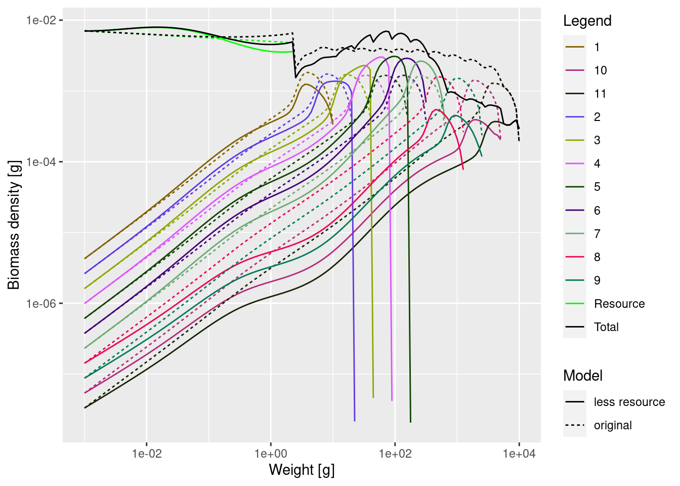
But we can also save and then display the spectra of all the species at intermediate times. This is what the project() function does. It projects the current state forward in time and saves the result of that simulation in a larger object, a MizerSim object, which contains the resulting time series of size spectra. Let’s use it to project forward by 24 years.
sim_lessRes <- project(mp_lessRes, t_max = 24)We can now use this MizerSim object in the animateSpectra() function to create an animation showing the change in the size spectra over time.
animateSpectra(sim_lessRes, total = TRUE, power = 2,
               ylim = c(1e-8, NA), wlim = c(1e-3, NA))
Go ahead, press the Play button.
Note, for some species size spectra at the largest size class drop all the way to very small values (e.g. 10^-7) and for others they stop higher. This is just a discretisation artifact and is not important. Try to ignore it.
Of course we can also get at the numeric values of the spectra at different times. First of all the function getTimes() gives the times at which simulation results are available in the MizerSim object:
getTimes(sim_lessRes) [1] 0 1 2 3 4 5 6 7 8 9 10 11 12 13 14 15 16 17 18 19 20 21 22 23 24The function N() returns a three-dimensional array (time x species x size) with the number density of consumers. To get for example the number density for the 2nd species after 5 years in the 1st size class we do
N(sim_lessRes)[6, 2, 1][1] 2.621407If the function getBiomass() is supplied with a MizerSim object then it returns an array (time x species) containing the biomass in grams at each time step for all species. So for example the biomass in grams of the 2nd species after 5 years is
getBiomass(sim_lessRes)[6, 2][1] 0.003434511The biomass time series can be plotted with plotBiomass():
plotBiomass(sim_lessRes)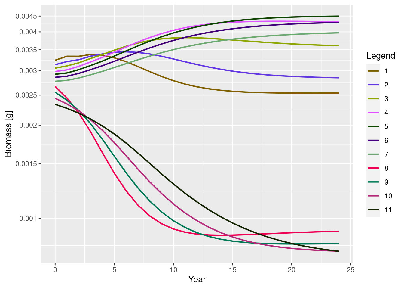
Mizer provides many more functions to analyse the results of a simulation, some of which you will learn later in this course.
Reproduction dynamics
The above simulation was run with constant abundance in the smallest size class for each species. This of course is not realistic. The abundance of the smallest individuals depends on the rate at which mature individuals spawn offspring, and this in turn depends, among other things, on the abundance of mature individuals. So if the abundance of mature individuals goes down drastically, as it did for species 8 to 11 above, then the abundance of offsprings for those species will go down as well.
To see the effect we run the same code as above after deleting the two lines that turned off the reproduction dynamics. We also specify with t_save = 2 that we want to save the spectrum only every second year, which speeds up the display of the animation.
# Create trait-based model
mp <- newTraitParams() |>
    # run to steady state with constant reproduction rate
    steady()
Convergence was achieved in 6 years.# We make a copy of the model
mp_lessRes <- mp
# and set the resource interaction to 0.8 for species 8 to 11
species_params(mp_lessRes)$interaction_resource[8:11] <- 0.8
# We simulate the dynamics for 30 years, saving only every 2nd year
sim_lessRes <- project(mp_lessRes, t_max = 30, t_save = 2)
# We animate the result
animateSpectra(sim_lessRes, total = TRUE, power = 2,
ylim = c(1e-8, NA), wlim = c(1e-3, NA))I think you might be surprised at the result when you press the Play button now.
What is going on with species 1?
How reproduction is modelled
Energy invested into reproduction
We already discussed the investment into reproduction in an earlier tutorial. As mature individuals grow they invest an increasing proportion of their income into reproduction and at their asymptotic size they would be investing all income into reproduction. Summing up all these investments from mature individuals of a particular species gives the total rate E_R at which that species invests energy into reproduction. This total rate of investment is multiplied by a reproduction efficiency factor erepro, divided by a factor of 2 to take into account that only females reproduce, and then divided by the egg weight w_min to convert it into the rate at which eggs are produced. The equation is:
R_{di} = \frac{\rm{erepro}}{2 w_{min}} E_R.
This is calculated in mizer with getRDI():
getRDI(mp) 1 2 3 4 5 6
0.344090412 0.211705188 0.130253809 0.080140004 0.049306967 0.030336622
7 8 9 10 11
0.018664921 0.011483786 0.007065518 0.004347133 0.002674619 The erepro parameter or reproduction efficiency can vary between 0 and 1 (although 0 would be bad) and reflects the fact that only a fraction of energy invested into reproduction can make into viable eggs or larvae.
Density-dependence in reproduction
Note that what mizer models is not the rate of recruitment but the rate of egg production. The size spectrum dynamics then determine how many of those larvae grow up and survive to be recruited to the fishery.
The stock-recruitment relationship is an emergent phenomenon in mizer, with several sources of density dependence. Firstly, the amount of energy invested into reproduction depends on the energy income of the spawners, which is density-dependent due to competition for prey. Secondly, the proportion of larvae that grow up to recruitment size depends on the larval mortality, which depends on the density of predators, and on larval growth rate, which depends on density of prey.
However there are other sources of density dependence that are not explicitly modelled mechanistically in mizer. An example would be a limited carrying capacity of suitable spawning grounds and other spatial effects. So mizer has another species parameter R_{max} that gives the maximum possible rate of recruitment. Imposing a finite maximum reproduction rate leads to a non-linear relationship between energy invested and eggs hatched. This density-dependent reproduction rate is given by a Beverton-Holt type function:
R_{dd} = R_{di} \frac{R_{max}}{R_{di} + R_{max}}
Rather than looking at the formula, let’s look at a figure:
Warning: Using `size` aesthetic for lines was deprecated in ggplot2 3.4.0.
ℹ Please use `linewidth` instead.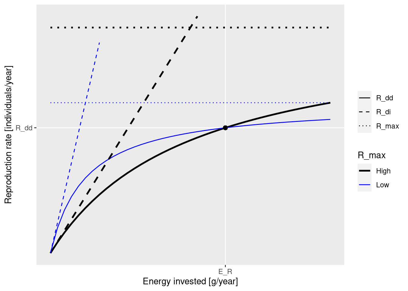
This figure shows two graphs of R_{dd} (solid lines), one for higher R_{max} (black) and one for lower R_{max} (blue). The values of R_{max} are indicated by the dotted lines. The dashed lines show the density-independent rate R_{di}.
The important fact to observe is that the solid curves becomes more shallow as R_{max} gets closer to the actual reproduction rate R_{dd}. This slope determines how big the effect of a change in investment into reproduction (for example due to a change in spawning stock biomass) is on the reproduction rate. As the energy invested in reproduction changes away from the steady state value E_R on the x-axis, the the solid curves shows how much the reproduction rate changes on the y-axis. The change is smaller along the shallower blue line, the one that corresponds to the R_{max} value that is closer to R_{dd}. The result is that a species with a low ration between R_max and R_{dd} will be less impacted by depletion of its spawning stock by fishing, for example. This ratio we will refer to as the reproduction level and we will discuss it in the next section.
This density-dependent rate of reproduction is calculated in mizer with getRDD():
getRDD(mp) 1 2 3 4 5 6
0.258067809 0.158778891 0.097690357 0.060105003 0.036980226 0.022752467
7 8 9 10 11
0.013998691 0.008612839 0.005299139 0.003260350 0.002005964 This is the rate at which new individuals are entering the smallest size class. The actual number density in the smallest size class is then determined by the usual size-spectrum dynamics.
Reproduction level
We have seen the two species parameters that determine how the energy invested into reproduction is converted to the number of eggs produced: erepro and R_max. For neither of these is it obvious what value they should have. The choice of values influences two important properties of a model: the steady state abundances of the species and the density-dependence in reproduction. It is therefore useful to change to a new set of two parameters that reflect these two properties better. These are:
The birth rate R_{dd} at steady state. This determines the abundance of a species.
The ratio between R_{dd} and R_{max} at steady state. This determines the degree of density dependence.
The ratio R_{dd} / R_{max} we denote as the reproduction level. This name may remind you of the feeding level, which was the ratio betweenthe actual feeding rate and the the maximum feeding rate and described the level of density dependence coming from satiation. It takes a value between 0 and 1. It follows from our discussion in the previous section that a species with a high reproduction level is more resilient to changes.
We can get the reproduction levels of the different species with getReproductionLevel():
   1    2    3    4    5    6    7    8    9   10   11
0.25 0.25 0.25 0.25 0.25 0.25 0.25 0.25 0.25 0.25 0.25
We see that by default newTraitParams() had given all species the same reproduction level. We can change the reproduction level with the setBevertonHolt() function. We can set different reproduction levels for each species, but here we will simply set it to 0.9 for all species:
mp9 <- setBevertonHolt(mp, reproduction_level = 0.9)Changing the reproduction level has no effect on the steady state, because that only depends on the rate of egg production R_dd and that is kept fixed when changing the reproduction level. We can check that by running our new model to steady state and plotting that steady state together with the original steady state. They overlap perfectly.
mp9 <- projectToSteady(mp9)Convergence was achieved in 3 years.plotSpectra2(mp, "reproduction_level = 0.25", mp9, "reproduction_level = 0.9",
total = TRUE, power = 2, ylim = c(1e-8, NA), wlim = c(1e-3, NA))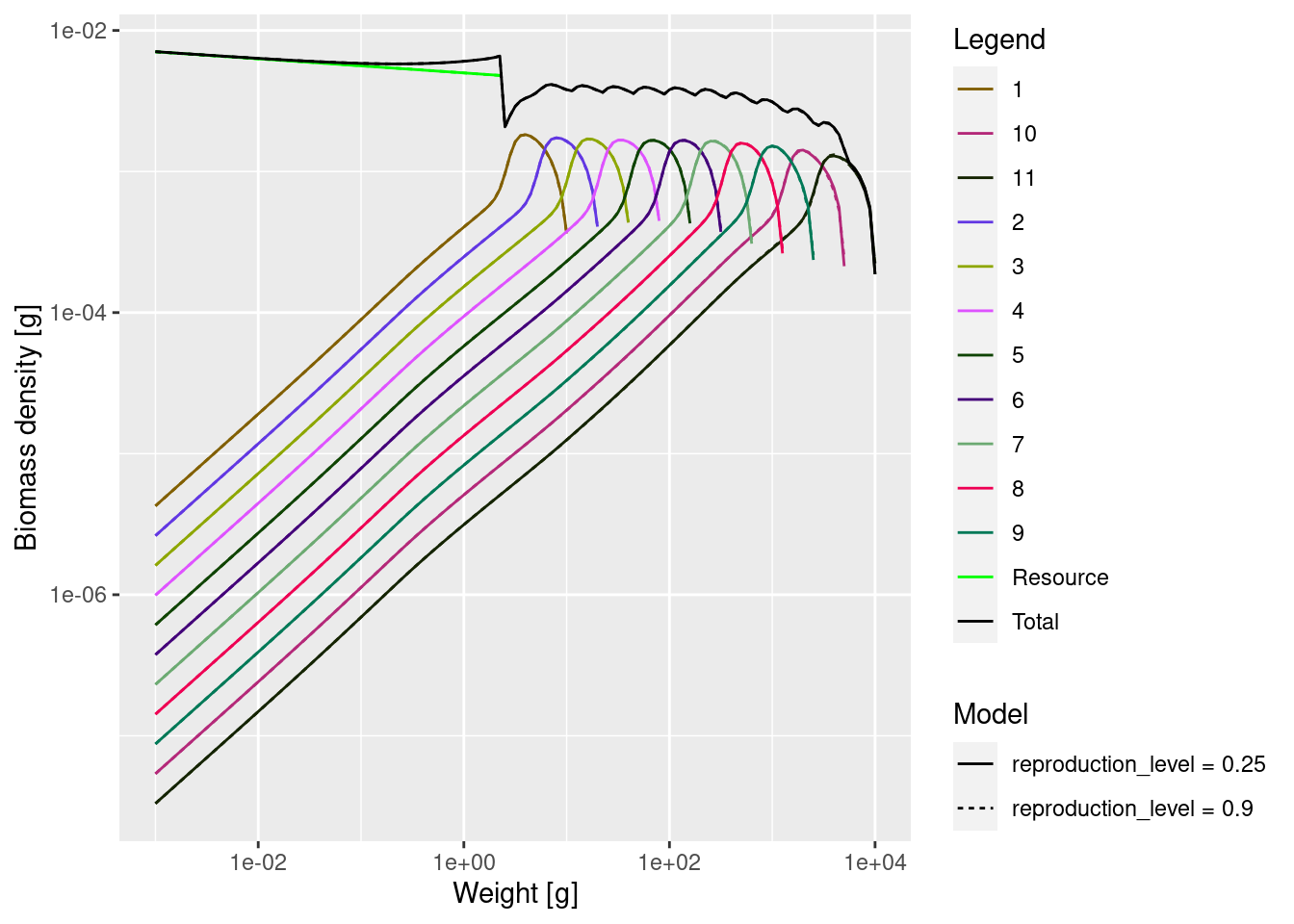
However the reproduction level has an effect on how sensitive the system is to changes. As an example, let us look at the dynamics that is triggered by the reduction in interaction with the resource by species 8 through 11.
# We make a copy of the model
mp_lessRes9 <- mp9
# and set the resource interaction to 0.8 for species 8 to 11
species_params(mp_lessRes9)$interaction_resource[8:11] <- 0.8

sim_lessRes9 <- project(mp_lessRes9, t_max = 30, t_save = 2)

animateSpectra(sim_lessRes9, total = TRUE, power = 2,
               ylim = c(1e-8, NA), wlim = c(1e-3, NA))
Notice how the species have settled down to a new steady state after 30 years without any extinctions and the impact on species 1 is almost negligible. As expected, the higher reproduction level has made the species much more resilient to perturbations.
The problem of course is that in practice the reproduction level is hardly ever known. Instead one will need to use any information one has about the sensitivity of the system from observed past perturbations to calibrate the reproduction levels. We’ll discuss this again in week 3.
Go back to the example with fishing on individuals above 1kg from the section on fishing-induced cascades. Impose the same fishing, but now on the trait-based model with reproduction dynamics left turned on and with a reproduction level of 0.5 for all species. Project the model for 20 years. How many species have a reduced total biomass after 20 years? What is the total biomass of species 1 after 20 years?
Resource dynamics
The resource spectrum is not described by size spectrum dynamics, because in reality it is typically not made up of individuals that grow over a large size range during their life time. In mizer, the resource number density in each size class is describe by semichemostat dynamics: the resource number density in each size class increases recovers after depletion, and this biomass growth or recovery rate will decrease as the number density gets close to a carrying capacity. If you want the mathematical details, you can find them in the mizer model description in the section on resource density.
The effect of these dynamics is that if the number of fish consuming the resource in a certain size range increases, the resource abundance in that size range will decrease, if it cannot recover quickly enough (regeneration rate of the resource is set by the user). So there is competition for the resource, which provides a stabilising influence on the fish abundances. We will be discussing this more in week 3.
Summary and recap
1) Size spectrum dynamics is very intuitive: the rate at which the number of individuals in a size class changes is the difference between the rate at which individuals grow into (or are born into) the size class and the rate at which individuals grow out of or the size class or die in the size class.
2) The project() function simulates the dynamics and creates a MizerSim object that contains the resulting time series of size spectra.
3) Mizer provides many functions for extracting, analysing and plotting the results of a simulation, some of which we will be using in week 3.
4) Instead of a stock-recruitment relationship as used in other fisheries models, a mizer model relates the energy invested into reproduction to the number of eggs produced. The growth and mortality that the larvae experience until they are recruited to the fishery lead to density-dependence in the recruitment. Additional density dependence is applied to the egg production.
5) The relation between energy invested in reproduction and the actual birth rate is described by two parameters: the density independent reproduction efficiency erepro and the maximum birth rate R_max.
6) In practice a more useful way to parametrise the reproduction is by two other parameters: the birth rate R_{dd} at steady state (which determines the total abundance of a species) and the reproduction level (which determines the amount the amount of density dependence that applies to egg production).
7) A change in the reproduction level does not change the steady state but it changes the sensitivity of a species and the system to changes.